How does physical activity level influence sleep quality across different age groups?
# Load necessary librarieslibrary(glmnet)
Warning: package 'glmnet' was built under R version 4.3.3
Loading required package: Matrix
Loaded glmnet 4.1-8
library(plotly)
Warning: package 'plotly' was built under R version 4.3.3
Loading required package: ggplot2
Attaching package: 'plotly'
The following object is masked from 'package:ggplot2':

    last_plot
The following object is masked from 'package:stats':

    filter
The following object is masked from 'package:graphics':

    layout
library(ggplot2)# Load the datasetdata1 <-read.csv("C:/Users/ACER/Desktop/New folder/Sai Sriram Uppada/FinalProject/Sleep_health_and_lifestyle_dataset.csv") # Replace with the path to the original dataset# Prepare the data# Assuming 'Quality_of_Sleep' is a continuous variable and both 'Age' and 'Physical_Activity_Level' are already numerical.x <-model.matrix(Quality.of.Sleep ~ Age * Physical.Activity.Level, data = data1)[, -1] # removing intercepty <- data1$Quality.of.Sleep# Fit Lasso Regression modellasso_model <-glmnet(x, y, alpha =1) # alpha = 1 for Lasso# Cross-validation for optimal lambdacv_lasso <-cv.glmnet(x, y, alpha =1)coef(lasso_model, s = cv_lasso$lambda.min)
4 x 1 sparse Matrix of class "dgCMatrix"
s1
(Intercept) -2.336480711
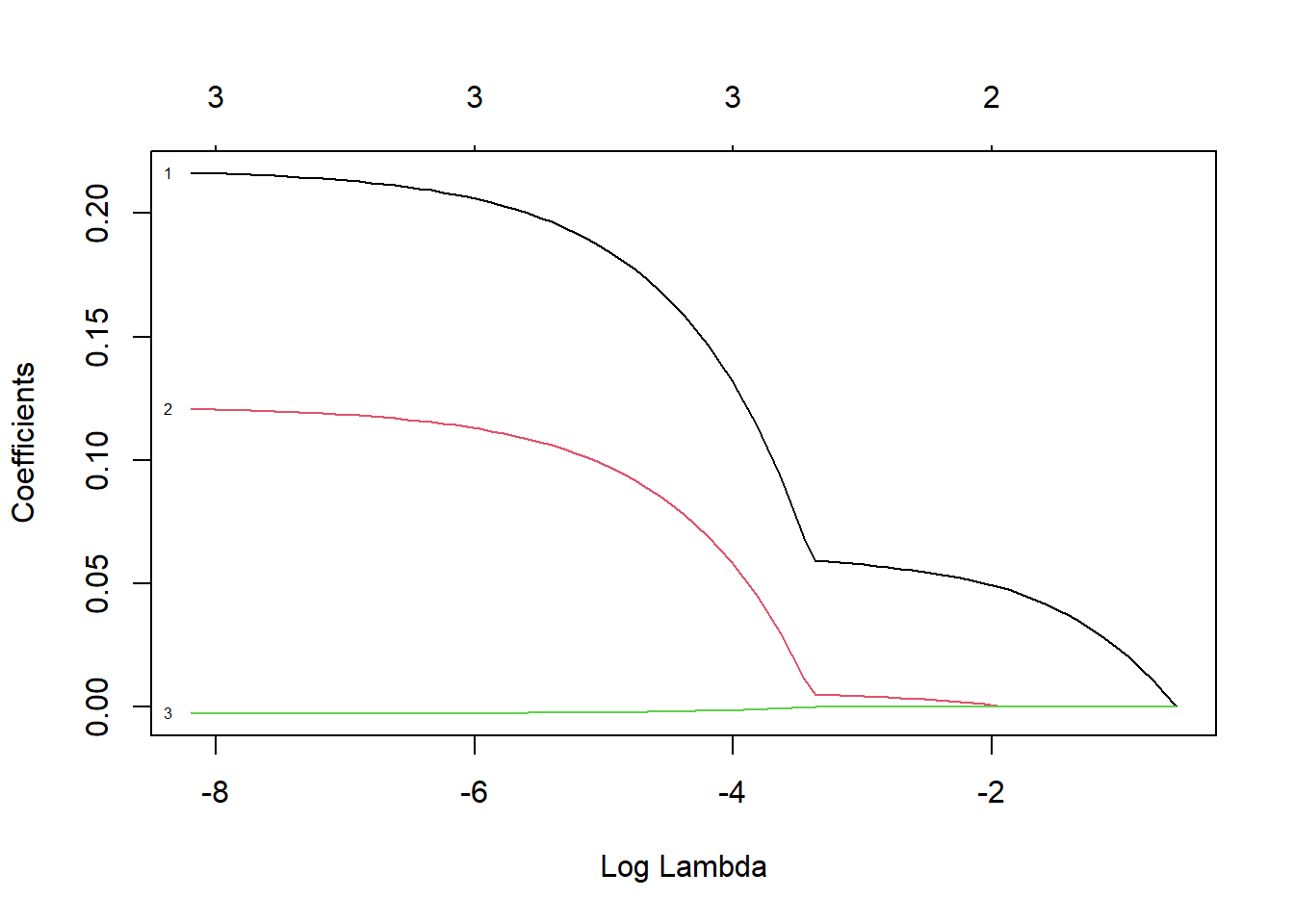
Age 0.216280398
Physical.Activity.Level 0.120627719
Age:Physical.Activity.Level -0.002615155
# Plotting the coefficient pathplot(lasso_model, xvar ="lambda", label =TRUE)
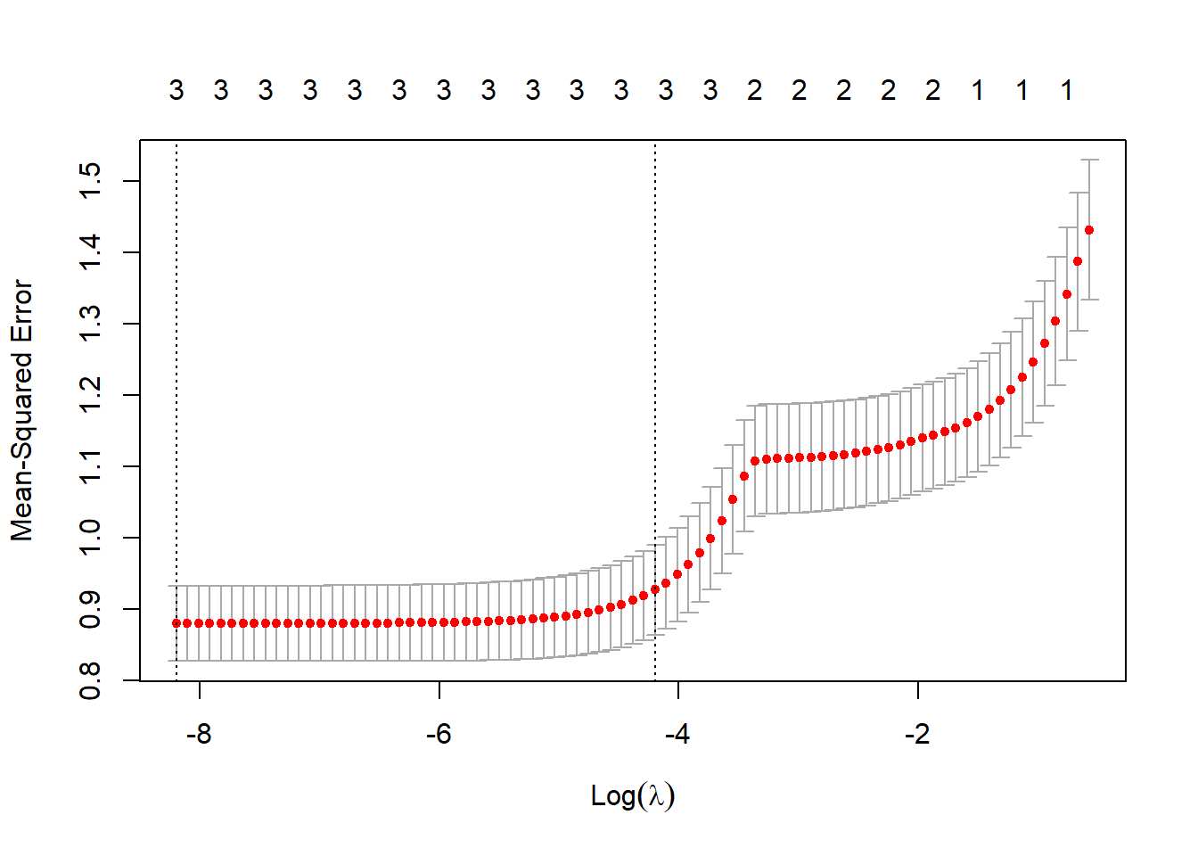
# Create a ggplot# Plotting cross-validation plot to see the optimal lambdaplot(cv_lasso)
# Creating a new data frame for predictionsage_range <-seq(min(data1$Age), max(data1$Age), by =1)pa_levels <-seq(min(data1$Physical.Activity.Level), max(data1$Physical.Activity.Level), length.out =100)# Creating a grid of Age and Physical Activity levelsgrid_data <-expand.grid(Age = age_range, Physical.Activity.Level = pa_levels)# Correcting newdata matrix generationgrid_data_matrix <-model.matrix(~ Age * Physical.Activity.Level, data = grid_data)[, -1]# Predicting using the correct newx argumentgrid_data$Quality_of_Sleep_Pred <-predict(lasso_model, newx = grid_data_matrix, s = cv_lasso$lambda.min)# Plottinga =ggplot(grid_data, aes(x = Age, y = Physical.Activity.Level, fill = Quality_of_Sleep_Pred)) +geom_tile() +scale_fill_gradient2(low ="blue", high ="red", mid ="white", midpoint =median(grid_data$Quality_of_Sleep_Pred), space ="Lab", name ="Predicted\nSleep Quality") +labs(x ="Age", y ="Physical Activity Level", title ="Predicted Sleep Quality Across Age and Physical Activity Levels") +theme_minimal() +theme(panel.grid.major =element_blank(), panel.grid.minor =element_blank())ggplotly(a)
RESEARCH QUESTION- 2
What are the key predictors influencing sleep quality, and how can we predict sleep quality based on lifestyle and health metrics?
library(randomForest)
Warning: package 'randomForest' was built under R version 4.3.3
randomForest 4.7-1.1
Type rfNews() to see new features/changes/bug fixes.
Attaching package: 'randomForest'
The following object is masked from 'package:ggplot2':

    margin
library(ggplot2)library(plotly)library(dplyr)
Attaching package: 'dplyr'
The following object is masked from 'package:randomForest':

    combine
The following objects are masked from 'package:stats':

    filter, lag
The following objects are masked from 'package:base':

    intersect, setdiff, setequal, union
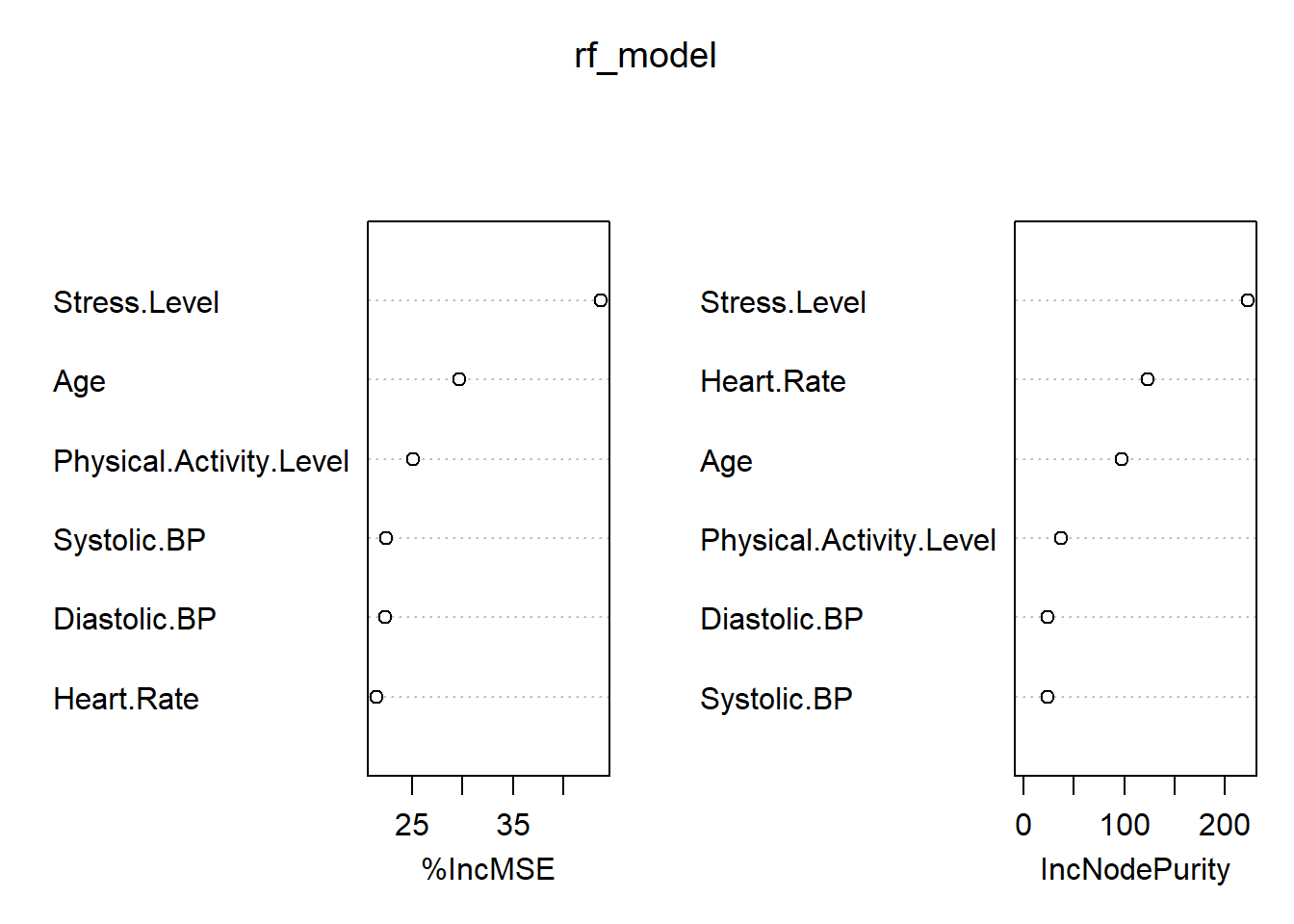
# Load the datasetdata1 <-read.csv("C:/Users/ACER/Desktop/New folder/Sai Sriram Uppada/FinalProject/Sleep_health_and_lifestyle_dataset.csv") # Replace with the path to the original dataset# Split the "Blood Pressure" into "Systolic BP" and "Diastolic BP"data1 <- data1 %>%mutate(Systolic.BP =as.integer(sub("/.*", "", Blood.Pressure)),Diastolic.BP =as.integer(sub(".*/", "", Blood.Pressure)))# Fit Random Forest model to predict sleep qualityset.seed(123) # for reproducibilityrf_model <-randomForest(Quality.of.Sleep ~ Age + Physical.Activity.Level + Stress.Level + Heart.Rate + Systolic.BP + Diastolic.BP, data=data1, importance=TRUE, ntree=500)# Check out the model summaryprint(rf_model)
Call:
 randomForest(formula = Quality.of.Sleep ~ Age + Physical.Activity.Level +      Stress.Level + Heart.Rate + Systolic.BP + Diastolic.BP, data = data1,      importance = TRUE, ntree = 500)
               Type of random forest: regression
                     Number of trees: 500
No. of variables tried at each split: 2

          Mean of squared residuals: 0.02697864
                    % Var explained: 98.11
# Predict sleep qualitypredicted_quality <-predict(rf_model, data1)# Create a plot of actual vs predicted sleep qualitydata1$Predicted_Quality_of_Sleep <- predicted_qualitya =ggplot(data1, aes(x=Quality.of.Sleep, y=Predicted_Quality_of_Sleep)) +geom_point(alpha=0.5) +geom_smooth(method='lm', color='red') +labs(x="Actual Sleep Quality", y="Predicted Sleep Quality", title="Actual vs Predicted Sleep Quality") +theme_minimal()# Convert ggplot object to an interactive plotly objectggplotly(a)
`geom_smooth()` using formula = 'y ~ x'
RESEARCH QUESTION- 3
Does BMI predict the presence of sleep apnea?
# Load necessary librarieslibrary(readr)
Warning: package 'readr' was built under R version 4.3.3
library(dplyr)library(glmnet)library(ggplot2)# Load the dataset (adjust the file path as needed)sleep_data <-read.csv("C:/Users/ACER/Desktop/New folder/Sai Sriram Uppada/FinalProject/Sleep_health_and_lifestyle_dataset.csv") # Rename columns if needed to match the code# Assuming "BMI.Category" is the column containing BMI informationcolnames(sleep_data) <-gsub("\\.", "_", colnames(sleep_data)) # Prepare the predictor variables and the response# Assuming "BMI_Category" is the column name for BMI informationsleep_data$Sleep_Apnea <-as.factor(ifelse(sleep_data$Sleep_Disorder =="Sleep Apnea", 1, 0))predictors <-model.matrix(~ BMI_Category, sleep_data)[, -1]response <- sleep_data$Sleep_Apnea# Fit logistic regression modelfit_apnea <-glmnet(predictors, response, family ="binomial")# Print coefficientscoef(fit_apnea)
Warning: package 'pROC' was built under R version 4.3.3
Type 'citation("pROC")' for a citation.
Attaching package: 'pROC'
The following objects are masked from 'package:stats':

    cov, smooth, var
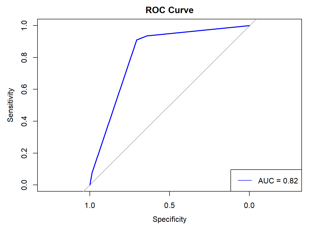
# Make predictions on the training setpredictions_train <-predict(cv_fit_apnea, type ="response", s ="lambda.min", newx = predictors)# Calculate ROC curveroc_curve <-roc(as.numeric(response) -1 , predictions_train)
Setting levels: control = 0, case = 1
Warning in roc.default(as.numeric(response) - 1, predictions_train): Deprecated
use a matrix as predictor. Unexpected results may be produced, please pass a
numeric vector.
Setting direction: controls < cases
# Plot ROC curve with AUCplot(roc_curve, main ="ROC Curve", col ="blue")legend("bottomright", legend =paste("AUC =", round(auc(roc_curve), 2)), col ="blue", lty =1)